AP Calculus BC Formula Sheet 2020 Edition

AP Calculus BC Formula Sheet 2020 Edition

The AP Calculus BC Formula Sheet provides essential formulas and theorems for students preparing for the AP Calculus BC exam. Key topics include the definition of derivatives, continuity, the Mean Value Theorem, and the Intermediate Value Theorem. This resource also outlines critical numbers, the first and second derivative tests, and concavity definitions. Designed for high school students, it serves as a quick reference for calculus concepts and problem-solving strategies. The sheet includes integration techniques, particle motion formulas, and methods for determining area and volume under curves.

Key Points

  • Includes definitions of derivatives and continuity essential for AP Calculus BC.
  • Covers the Mean Value Theorem and Intermediate Value Theorem for function analysis.
  • Explains critical numbers and the first and second derivative tests for identifying extrema.
  • Details particle motion equations and their applications in real-world scenarios.
211
/ 5
2020 AP CALCULUS BC FORMULA LIST
______________________________________________________________________________
Definition of the derivative:
0
( ) lim
h
f x h f x
fx
h

lim
xa
f x f a
fa
xa
(Alternative form)
____________________________________________________________________________
Definition of continuity: f is continuous at c if and only if
1) f (c) is defined;
2)
lim ( ) exists;
xc
fx
3)
lim ( ) ( ).
xc
f x f c
____________________________________________________________________________________________________
Mean Value Theorem: If f is continuous on [a, b] and differentiable on (a, b), then there
exists a number c on (a, b) such that
( ) .
f b f a
fc
ba
_____________________________________________________________________________________________________
Intermediate Value Theorem: If f is continuous on [a, b] and k is any number between f (a)
and f (b), then there is at least one number c between a and b such that f (c) = k.
_____________________________________________________________________________________________________
1
2
11
2
nn
du
d d d
dx
x nx u
dx dx dx x x
u







2
f x g x f x f x g x
dd
f x g x f x g x g x f x
dx dx g x
gx
d
f g x f g x g x
dx









[sin ] cos [cos ] sin
d du d du
u u u u
dx dx dx dx
[sec ] sec tan [csc ] csc cot
d du d du
u u u u u u
dx dx dx dx
11
[ln ] [log ]
ln
a
d du d du
uu
dx u dx dx u a dx

[ ] [ ] ln
u u u u
d du d du
e e a a a
dx dx dx dx

22
11
[arcsin ] [arccos ]
11
d du d du
uu
dx dx dx dx
uu

22
11
[arctan ] [arccot ]
11
d du d du
uu
dx u dx dx u dx

____________________________________________________________________________________________
Definition of a definite integral:
0
11
lim lim
nn
xn
k k k k
kk
b
a
f x dx f x x f x x


cos sin sin cosu du u C u du u C

1
,1
1
n
n
x
x dx C n
n
1
lndu u C
u

ln
u
u u u
a
e du e C a du C
a

f g x g x dx f g x C

____________________________________________________________________________________________
Definition of a Critical Number:
Let f be defined at c. If
0 or if f c f

is undefined at c, then c is a critical number of f.
_______________________________________________________________________
First Derivative Test:
Let c be a critical number of a function f that is continuous on an open interval I
containing c. If f is differentiable on the interval, except possibly at c, then
fc
can be classified:
1) If
fx
changes from negative to positive at c, then
,c f c
is a relative
minimum of f.
2) If
fx
changes from positive to negative at c, then
,c f c
is a relative
maximum of f.
Second Derivative Test:
Let f be a function such that the second derivative of f exists on an open interval containing c.
1) If
0fc
and
0fc

, then
,c f c
is a relative minimum.
2) If
0fc
and
0fc

, then
,c f c
is a relative maximum
______________________________________________________________________________
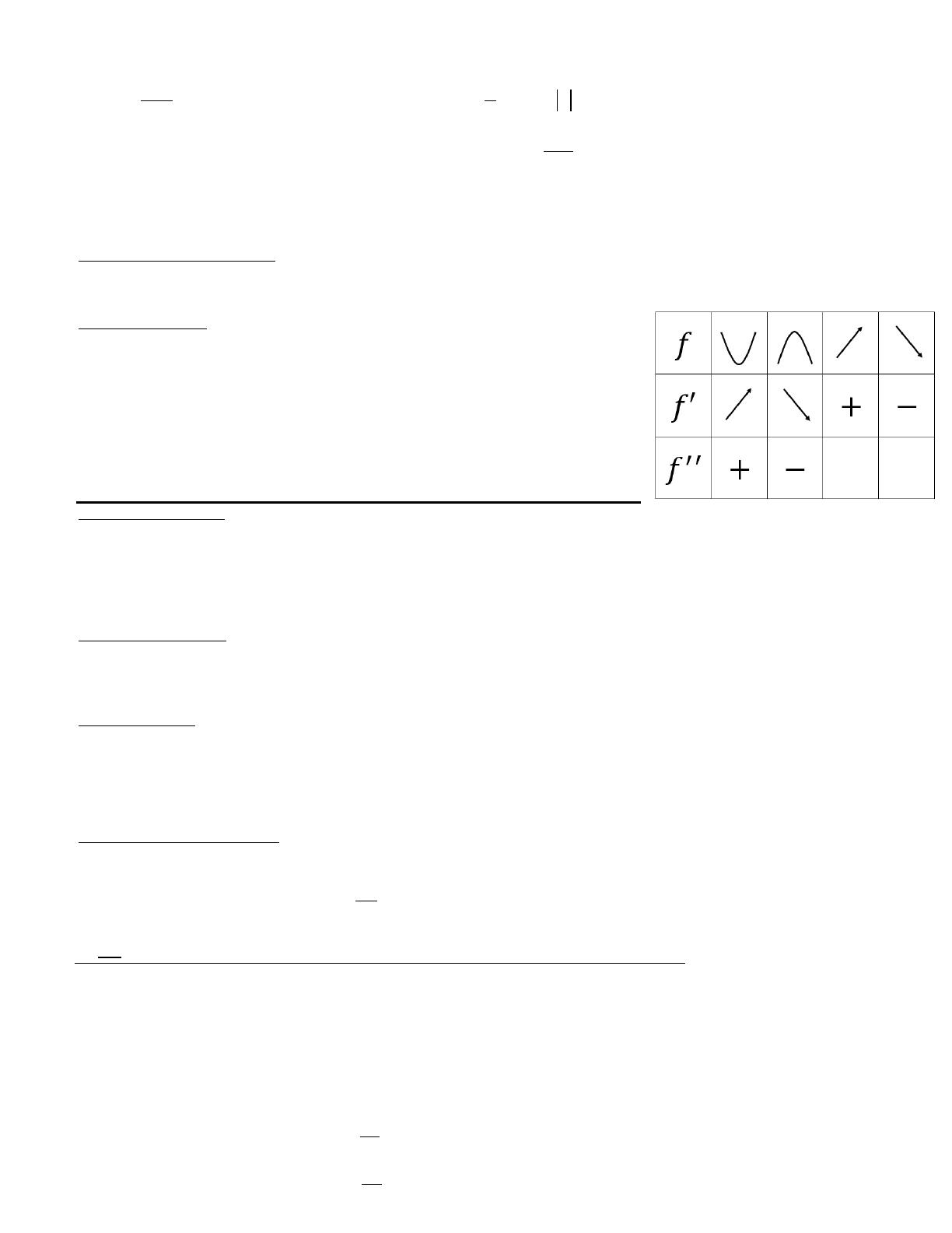
Definition of Concavity:
Let f be differentiable on an open interval I. The graph of f is concave upward on I if
f
is increasing on the interval and
concave downward on I if
f
is decreasing on the interval.
______________________________________________________________________________
Test for Concavity:
Let f be a function whose second derivative exists on an open interval I.
1) If
0fx

for all x in I, then the graph of f is concave upward in I.
2) If
0fx

for all x in I, then the graph of f is concave downward in I.
______________________________________________________________________________
Definition of an Inflection Point:
A function f has an inflection point at
,c f c
1) if
0 or f c f c
does not exist and
2) if
f

changes sign from positive to negative or negative to positive at
xc
OR if
fx
changes from increasing to decreasing or decreasing to increasing at x = c.
First Fundamental Theorem of Calculus:
b
a
f x dx f b f a

final initial + change
initial final change
b
a
b
a
f b f a f x dx
f a f b f x dx
Second Fundamental Theorem of Calculus:
x
a
d
f t dt f x
dx
Chain Rule Version:
gx
a
d
f t dt f g x g x
dx

Average rate of change of f (x) on [a, b]:
_____________________________________________________________________________________________
Average value of f (x) on [a, b]:
1
()
b
AVE
a
f f x dx
ba
______________________________________________________________________________________________
Particle Motion
If an object moves along a straight line with position function
st
, then its
Velocity is
v t s t
Speed =
vt
Acceleration is
a t v t s t

Displacement (change in position) from
to x a x b
is Displacement =
b
a
v t dt
Total Distance traveled from
to x a x b
is Total Distance =
b
a
v t dt
At rest means
0.vt
An object is moving left (down) when
0vt
and an object is moving right (up) when
0.vt
An object changes direction when velocity changes signs.
An object is speeding up when velocity and acceleration have the same sign.
An object is slowing down when velocity and acceleration have different signs.
________________________________________________________________________________________
Rate In/Rate Out
rate of change = amount of change from to
b
a
dt t a t b
00
( ) initial amount + amount in - amount out
( ) = initial amount + rate in rate out
tt
At
A t dt dt

amount rate
d
dt
If rate in > rate out, then amount is increasing
If rate out > rate in, then amount is decreasing
When finding abs max and/or abs max, use candidates test. To find critical values: rate in = rate out.
______________________________________________________________________________
L’Hospital’s Rule:
Suppose that
f
and
g
are differentiable functions and that
( ) 0gx
near
xa
and
lim ( ) 0 and lim ( ) 0
x a x a
f x g x


or that
lim ( ) and lim ( )
x a x a
f x g x

 
Then
( ) ( )
lim lim
( ) ( )
x a x a
f x f x
g x g x

/ 5
End of Document
211
You May Also Like
Faqs of AP Calculus BC Formula Sheet 2020 Edition
What are the key formulas included in the AP Calculus BC Formula Sheet?
The AP Calculus BC Formula Sheet includes essential formulas such as the definition of the derivative, continuity conditions, and the Mean Value Theorem. It also provides formulas for integration techniques, including integration by parts and the disk and washer methods for calculating volumes. Additionally, it covers the first and second derivative tests, which are crucial for identifying relative extrema and concavity in functions. This comprehensive collection supports students in mastering calculus concepts for the AP exam.
How does the Mean Value Theorem apply in calculus?
The Mean Value Theorem states that if a function is continuous on a closed interval [a, b] and differentiable on the open interval (a, b), then there exists at least one point c in (a, b) where the derivative of the function equals the average rate of change over that interval. This theorem is fundamental in understanding the behavior of functions and is often used to prove other important results in calculus. It helps students analyze function behavior and apply calculus concepts to real-world problems.
What is the significance of critical numbers in calculus?
Critical numbers are points in the domain of a function where the derivative is either zero or undefined. These points are significant because they can indicate potential local maxima or minima of the function. By applying the first and second derivative tests at these critical numbers, students can determine the nature of these points and analyze the overall behavior of the function. Understanding critical numbers is essential for optimizing functions in various applications.
What methods are used to calculate the area under a curve?
Calculating the area under a curve can be achieved using several methods, including the disk method and the washer method. The disk method is used when the region is revolved around a horizontal axis, while the washer method accounts for areas with holes in the shape. Both methods involve integrating the function that describes the curve over a specified interval. These techniques are crucial for solving problems related to volume and area in calculus.
What role does the second derivative test play in analyzing functions?
The second derivative test is used to determine the concavity of a function and to classify critical points found using the first derivative. If the second derivative at a critical point is positive, the function is concave up, indicating a local minimum. Conversely, if the second derivative is negative, the function is concave down, suggesting a local maximum. This test is a powerful tool for understanding the behavior of functions and is widely applied in optimization problems.